
- Simulations are relatively simple, inexpensive, and everything can be measured in principle.
- Not to reproduce experimental results (exception: testing the accuracy of potentials)
- Help to understand experimental results or to propose new experiments
- Test of theoretical predictions or theories
Using bash variables in sed command
Bash commands such as awk and sed are very handy tools when dealing with text files. For example, if line 30~70 in a pw.out file are the atom coordinates, we can simply type in the terminal:
and line 30~70 will show up on the terminal.
Things get tricker when the line numbers are variables. Often times we want to use sed in a bash script, and we need to use bash variables. However sed doesn't understand the normal bash variable substituion: $variable. For example, bash doesn't recognize: sed -n '${linehead},${linetail}p' file.
I got stuck on this for a while and more than one time, so I decided to write it down here. The way to get around is to first created a string that contains the whole sed argment (sedarg below), and put the whole string after sed command with eval in front.
There you go. I love sed. I could've loved it even more if this wasn't an issue.
Variable substitution in awk is totally another issue (which is as annoying). I will write it down next time when I have to google it again.
|
$ sed -n '30,70' pw.out |
and line 30~70 will show up on the terminal.
Things get tricker when the line numbers are variables. Often times we want to use sed in a bash script, and we need to use bash variables. However sed doesn't understand the normal bash variable substituion: $variable. For example, bash doesn't recognize: sed -n '${linehead},${linetail}p' file.
I got stuck on this for a while and more than one time, so I decided to write it down here. The way to get around is to first created a string that contains the whole sed argment (sedarg below), and put the whole string after sed command with eval in front.
|
#!/bin/bash sedarg="-e ${line_head,${linetail}p' file eval sed -n "$sedarg" |
There you go. I love sed. I could've loved it even more if this wasn't an issue.
Variable substitution in awk is totally another issue (which is as annoying). I will write it down next time when I have to google it again.
[VMD] Run vmd from Mac terminal
Our work can be done faster and more efficiently if we do everything through the terminal.
To ask vmd to open a file through MacOS X terminal, just type in:

Of course, I prefer a shorter version of the command vmd. Add the alias below to the .bashrc:
Now we are set to run vmd on Mac terminal. To open a .pdb file directly using vmd:
[New!]
To load a saved vmd state:
|
$/Applications/VMD\ 1.9.1.app/Contents/Resources/VMD.app/Contents/MacOS/VMD |
Of course, I prefer a shorter version of the command vmd. Add the alias below to the .bashrc:
|
alias vmd='/Applications/VMD\ 1.9.1.app/Contents/Resources/VMD.app/Contents/MacOS/VMD' |
Now we are set to run vmd on Mac terminal. To open a .pdb file directly using vmd:
|
$vmd openthis.pdb |
[New!]
To load a saved vmd state:
|
$vmd -e saved_state.vmd |
[LAMMPS] Visualizing log file
 (About how to use Pizza.py, please refers to previous post of How to use Pizza.py for LAMMPS or the official Pizza.py Toolkit page.
Instead of asking pizza.py to get all the "Temp", "TotEng" .. by typing in each variable, and then do g.plot (a lot of repetitive keyboard work!), there's a much faster way to visualize the thermo-type data. It allows us to quickly view the trend of properties, and get an idea of the equilibrium status of the simulation.
This can be done directly on the shell or through pizza.py. Below is to do it in pizza.py:
(About how to use Pizza.py, please refers to previous post of How to use Pizza.py for LAMMPS or the official Pizza.py Toolkit page.
Instead of asking pizza.py to get all the "Temp", "TotEng" .. by typing in each variable, and then do g.plot (a lot of repetitive keyboard work!), there's a much faster way to visualize the thermo-type data. It allows us to quickly view the trend of properties, and get an idea of the equilibrium status of the simulation.
This can be done directly on the shell or through pizza.py. Below is to do it in pizza.py:
| $ python -i /home/pizza/src/pizza.py |
| Pizza.py (9 Feb 2012), a toolkit written in Python type ? for help, CTRL-D to quit Loading tools ... >@run logview.py gnu log* Executing file: /home/pizza/scripts/logview.py 200000 read 10001 log entries |
[awk] using shell variable
Shell variable can be ported into awk command by using "-v" flag:
An important note here is that within the awk command, calling the var does not require the '$' sign.
If there are more than one shell variable to call, use -v again and put space in between:
This will print $1*$var and $var2.
|
#!/bin/bash var=100 awk -v var=$var '{print $1*var}' file.dat |
If there are more than one shell variable to call, use -v again and put space in between:
|
awk -v var=$var -v var2=$var2 '{print $1*var, var2}' file.dat |
How to converge ecut and kpoint in a DFT calculation?
Finding the energy cutoff and k-point is like the fundamental of doing DFT calculations. However there doesn't seem to be an universal way to do it. I found on the quantum-espresso forum a very informative and thorough explanation. Thank Stefano for a such detailed post. Below is my notes on the procedures:
1. First test ecutwfc and ecutrho
Ecutwfc and ecutrho are properties related to the Fourier components that are needed to describe the wavefunctions and the density of the system. The convergence depends on the highest Fourier components. Each pseudopotential has a required cutoff: the upperbound. The cutoff needed for a system containing several species is the highest among those needed for each element.
- Increasing ecutwfc value while fixing ecutrho = 4*ecutwfc. Perform total energy (if possibly, force and stress) convergence tests until satisfactory stability is reached[1].
2. Fix the ecutrho from Step 1, and reduce ecutwfc. See how much ecutwfc can be reduced without deteriorating the convergence.
3. Fix ecutwfc from step 2 and ecutrho from step 1, identify appropriate k-point.
- This one is tricker because convergence with respect to k-points is a property of the band structure. There is a big difference between convergence in a band insulator and in a metal.
(I don't quite understand this part, but it seems like in an insulator, the k-point convergence is rather simple comparing to a metal. In an insulator, bands are completely occupied or empty across the Brillouin zone and charge density can be written in terms of wannier functions that are exponentially localized in real space. As a result, the convergence with respect to the density of point in the different directions in the Brillouin zone should be exponentially fast and quick. On the other hand, metals require much denser set of k points in order to locate accurately the Fermi surface. This induces that a smearing width smoothing the integral to be performed.... )
[1] Satisfactory stability is typically ~0.05 eV/atom for energy, and 10meV/A for forces. (Or ~1 mry/atom and 1.e04 ry/au in atomic units)
[Mac] Set double-sided printing as default
I recently migrated from Windows to OSX. As a kinda-happy windows user for 20+ years, I was interested in knowing what's the charisma of Apple products.
--- Above is a totally unrelated preface ----------
In the System preference, there's no option to set duplex printing as default. Instead, Apple uses the Common Unix Printing System (CUPS) to manage the network printers. To access the printer settings, open a internet browser and go to http://127.0.0.1:631/printer. From the web-based interface, click on the name of the printer you want to set duplex printing. Two drop down menus here will allow you to do maintenance and administration tasks to this printer.
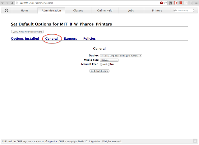
To set duplex printing, choose "Set Default Options" under the administration drop down menu. Click the "General" tab, and the Duplex setting will then show up. Choose 2-Sided, Long-Edge Binding (if you usually print the portrait orientation), and click on "Set Default Options".
The two-sided block should be always checked when you are trying to print. If not, try to restart the computer to clear memory of the printer settings in the applications.
Do more with the printer and the CUPS: http://127.0.0.1:631/admin
--- Above is a totally unrelated preface ----------
In the System preference, there's no option to set duplex printing as default. Instead, Apple uses the Common Unix Printing System (CUPS) to manage the network printers. To access the printer settings, open a internet browser and go to http://127.0.0.1:631/printer. From the web-based interface, click on the name of the printer you want to set duplex printing. Two drop down menus here will allow you to do maintenance and administration tasks to this printer.
To set duplex printing, choose "Set Default Options" under the administration drop down menu. Click the "General" tab, and the Duplex setting will then show up. Choose 2-Sided, Long-Edge Binding (if you usually print the portrait orientation), and click on "Set Default Options".
The two-sided block should be always checked when you are trying to print. If not, try to restart the computer to clear memory of the printer settings in the applications.
Do more with the printer and the CUPS: http://127.0.0.1:631/admin
[LAMMPS] Read/Observe Log File
Although we could always write our own scripts to process LAMMPS output files, LAMMPS has this awesome package, Pizza.py , which already contains many powerful tools to allow quick observations on the simulation results.
At the beginning of a simulation, you might want to check how energies and temperature drift, get averages over blocks of trajectory, and visualize the fluctuation of the simulation box. All these information can be retrieved in the log file, and all we need is the Pizza.py toolkit. Since the whole package is a combination of Python scripts, we also need to have Python installed.
Download the Pizza.py toolkit from this page , and put it in your directory. After unzipping it, you could find the Python script pizza.py in the src folder. The Pizza.py toolkit can be used directly or interactively.
First set up an alias pointing to where you put the pizza.py file. For example:
Then run pizza.py by typing in
This will bring you into the pizza.py interactive interface:
There might be some error messages after Loading tools if you don't have some of the modules required. Don't worry if you are missing some modules. Not every function uses all the modules.
Here I want to demonstrate how to use the interactive interface to observe the thermo output in LAMMPS log file.
This function will read in the files that have names end with log. This command calls the log.py script in the src folder. It can take multiple files, single files, even incomplete files. Check the comments in log.py to get more information.
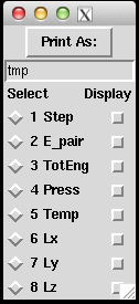
After reading in the thermo info stored in *log, we can get individual items. For example, to get timestep, pressure, temperature, energy:
Variables on the left hand side can just be any variables. The items inside the right hand parenthesis have to match with their names in the *log files.
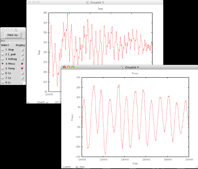
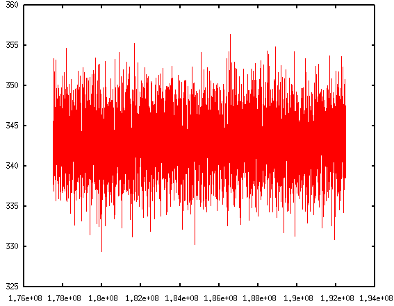
The thermo information fluctuates a lot. A better way to look at them is to plot against time. In the Pizza.py toolkit, they incorporate Gnuplot (in gnu.py) so that we can directly use it in the interactive interface:
The first command calls Gnuplot and the second command will plot timesteps vs. temperature.
 If you are like me, impatient of typing in those commands repetitively, don't worry. Pizza.py toolkit can also take scripts. There is a collection of scripts written by Pizza.py users. They come within the Pizza.py package. These scripts are handy to use and are very powerful. It allows me to do block averages in just one line.
Read more:
Block average
Visualizing log files
If you are like me, impatient of typing in those commands repetitively, don't worry. Pizza.py toolkit can also take scripts. There is a collection of scripts written by Pizza.py users. They come within the Pizza.py package. These scripts are handy to use and are very powerful. It allows me to do block averages in just one line.
Read more:
Block average
Visualizing log files
| $ alias pizza='python -i /home/pizza/src/pizza.py |
| $ pizza |
| Pizza.py (9 Feb 2012), a toolkit written in Python type ? for help, CTRL-D to quit Loading tools ... > |
| > l=log("*log") 180000000 182500000 185000000 187500000 190000000 192500000 read 6001 log entries |
| s,t,p,E=l.get("Step","Temp","Press","TotEng") |
| > g=gnu() > g.plot(s,t) |
If you are like me, impatient of typing in those commands repetitively, don't worry. Pizza.py toolkit can also take scripts. There is a collection of scripts written by Pizza.py users. They come within the Pizza.py package. These scripts are handy to use and are very powerful. It allows me to do block averages in just one line.
Read more:
Block average
Visualizing log files[GNUPLOT] Hide axis range
In gnuplot, a handy way to turn off the axis is to use:
This will remove all the tics and associated labels on the y axis.
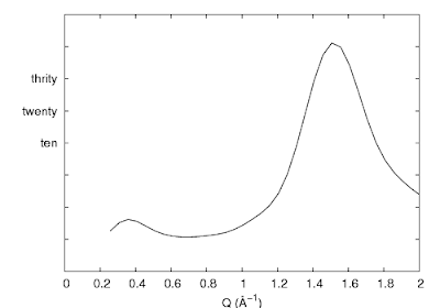
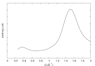
Sometimes we like to have the tics there, but hide just the numbers (i.e. when using arbitrary unit). A more complicated way is to use the set ytics ("〈label〉" 〈position〉,) command. This is used for assigning specific labels at given positions.
So utilizing this command, we could hide all the labels by removing the text inside the double quotes. Or, a much simpler way is to use set format:
Leave the double quotes empty will remove all the labels but keep the tics there.
| unset ytics |
| set ytics ("" -40, "" -30, "" -20, "" -10, "" 0, "ten" 10, "twenty" 20, "thrity" 30, "" 40, "" 50, "" 60) |
So utilizing this command, we could hide all the labels by removing the text inside the double quotes. Or, a much simpler way is to use set format:
| set format y "" |
Subscribe to:
Posts (Atom)