[LAMMPS] Read/Observe Log File

Although we could always write our own scripts to process LAMMPS output files, LAMMPS has this awesome package, Pizza.py , which already contains many powerful tools to allow quick observations on the simulation results.

At the beginning of a simulation, you might want to check how energies and temperature drift, get averages over blocks of trajectory, and visualize the fluctuation of the simulation box. All these information can be retrieved in the log file, and all we need is the Pizza.py toolkit. Since the whole package is a combination of Python scripts, we also need to have Python installed.

Download the Pizza.py toolkit from this page , and put it in your directory. After unzipping it, you could find the Python script pizza.py in the src folder. The Pizza.py toolkit can be used directly or interactively.

First set up an alias pointing to where you put the pizza.py file. For example:

$   alias pizza='python -i /home/pizza/src/pizza.py

Then run pizza.py by typing in

$   pizza

This will bring you into the pizza.py interactive interface:

Pizza.py (9 Feb 2012), a toolkit written in Python type ? for help, CTRL-D to quit Loading tools ... >

There might be some error messages after Loading tools if you don't have some of the modules required. Don't worry if you are missing some modules. Not every function uses all the modules.

Here I want to demonstrate how to use the interactive interface to observe the thermo output in LAMMPS log file.

>  l=log("*log") 180000000 182500000 185000000 187500000 190000000 192500000 read 6001 log entries

This function will read in the files that have names end with log. This command calls the log.py script in the src folder. It can take multiple files, single files, even incomplete files. Check the comments in log.py to get more information.

After reading in the thermo info stored in *log, we can get individual items. For example, to get timestep, pressure, temperature, energy:

s,t,p,E=l.get("Step","Temp","Press","TotEng")

Variables on the left hand side can just be any variables. The items inside the right hand parenthesis have to match with their names in the *log files.

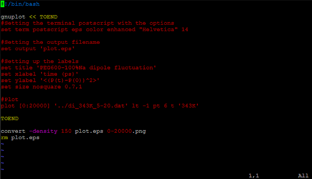
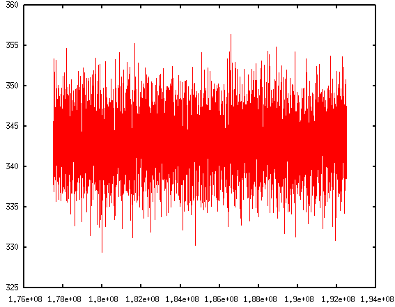
The thermo information fluctuates a lot. A better way to look at them is to plot against time. In the Pizza.py toolkit, they incorporate Gnuplot (in gnu.py) so that we can directly use it in the interactive interface:

> g=gnu() > g.plot(s,t)

The first command calls Gnuplot and the second command will plot timesteps vs. temperature.

If you are like me, impatient of typing in those commands repetitively, don't worry. Pizza.py toolkit can also take scripts. There is a collection of scripts written by Pizza.py users. They come within the Pizza.py package. These scripts are handy to use and are very powerful. It allows me to do block averages in just one line.

Read more:
Block average
Visualizing log files

[GNUPLOT] Hide axis range

In gnuplot, a handy way to turn off the axis is to use:

unset ytics

This will remove all the tics and associated labels on the y axis. Sometimes we like to have the tics there, but hide just the numbers (i.e. when using arbitrary unit). A more complicated way is to use the set ytics ("〈label〉" 〈position〉,) command. This is used for assigning specific labels at given positions.

set ytics ("" -40, "" -30, "" -20, "" -10, "" 0, "ten" 10, "twenty" 20, "thrity" 30, "" 40, "" 50, "" 60)

So utilizing this command, we could hide all the labels by removing the text inside the double quotes. Or, a much simpler way is to use set format:

set format y ""

Leave the double quotes empty will remove all the labels but keep the tics there.

Gnuplot with script

Gnuplot is a software in Linux machine that let you plot and fit your data.  It has an interactive interface, or if you prefer, you can plot data with a script.

Here's an example of a script that plot a file in postscript, and convert it into png file: The communication with gnuplot is enclosed by the two "TOEND". In side the TOEND, type in all the commands that you'd like gnuplot to do for you. If you'd like to use linux command to manipulate your data, i.e. awk, you'll have to add "\" when you use the "$" sign. For example if I want to make the x values 1000 times smaller :

plot "<awk '{print \$1/1000, \$2}' input_file"

Otherwise, if you only have "$1", the compiler will think it is the variable of the script itself.

After create the image in postscript format, the convert command (ImageMagick) could convert .eps files into .png files. The size of the png file can be controlled by the -density option.

This is really handy and makes the png plot in one press of enter.

---

[ Update 03/07/2012 ]
The 'convert' command is within the ImageMagick. With the update of ImageMagick to 6.7.5-10, extra arguments are required to create a PNG file with white background and smooth text.

convert -background white -alpha remove -density 150 plot.eps ${outputfile}

The default background for converting to PNG seems to be transparent in the latest ImageMagick (6.7.5-10). We need to remove the transparency (alpha) channel (-alpha remove), and assign the background to white (-background white).